Small Multiples Are Quick and Easy
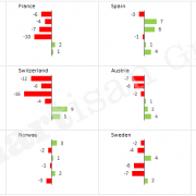
One of our previous posts discussed small multiples, i.e. a series of charts consisting of several small charts of the same type. It also describes conceptual considerations on typical application scenarios involving small multiples.
This post introduces an alternative method which you can use to create small multiples for simpler application scenarios at the blink of an eye. This type of alternative is especially interesting if the speed of implementation is more important that a special, individual chart design.
The idea: Excel sparklines are ‘opened up’ into a small multiple.
Sparklines are very simple diagrams nested within a single cell. Generally speaking, several of these charts are bundled together in a group, for which certain properties are defined, e.g. column colour or axis length. Use the following steps to transform standard sparklines into small multiples in a matter of minutes.
- “Insert” menu -> Sparklines -> Column / select data and location range so the sparklines appear next to the input area for the values
- Link the first sparkline with the first country name / copy the formula downwards for the other sparklines
- Move the cells with sparklines into a cell range with the desired layout
The interim result doesn’t provide a good overview over the data yet because Excel automatically displays each sparkline with an individual axis. Therefore, the charts need to be given a standardised axis using the following option:
- Click on a sparkline / “Design” menu -> Axis / set Minimum and Maximum value to the same for all sparklines
To increase the informational value, if required, you can also automatically display certain columns in a different colour, e.g. High Point and Last Point.
Done 🙂


